Non-transitive Grime Dice, via Mathematica

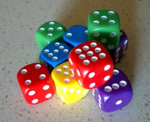
For Christmas this year, I got myself a fun mathematical gift: a set of 10 non-transitive dice, namely Grime Dice! You can get your own set here. Behold their dicey splendor:

These dice possess the fascinating property that their winning relationships (in the sense of “winning” = “rolls a higher number > 50% of the time”) are non-transitive. i.e. if die A wins against die B, and die B wins against die C, it actually does *not* hold, in general, that die A wins against die C.  In fact, die C might win against die A!

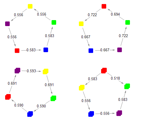
If we label the 5 Grime Dice colors Red, Blue, Yellow, Olive, and Magenta, there are 2 primary non-transitive winning cycles

1. By word length: Red beats Blue beats Olive beats Yellow beats Magenta beats Red
2. Alphabetically: Blue beats Magenta beats Olive beats Red beats Yellow beats Blue

That’s pretty neat and non-intuitive by itself, but things get weirder when you roll two dice of the same color together: the word length cycle reverses, while the alphabetical cycle (almost) stays intact.

1. By word length (doubles): Red/Red loses to Blue/Blue loses to Olive/Olive loses to Yellow/Yellow loses to Magenta/Magenta loses to Red/Red
2. Alphabetically (doubles): Blue/Blue beats Magenta/Magenta beats Olive/Olive loses to Red/Red beats Yellow/Yellow beats Blue/Blue

Using Mathematica, we can calculate the winning probabilities, and visualize the cycles:

These 4 cycles are the only ones which are advertised, but it turns out there are many more that you can form using just the 10 dice included in the set.

In fact, there are 298 such cycles! Here are the plots of all 1-die cycles,  all 2-dice cycles, and all 3-die cycles.

In this post, we’ll walk through the Mathematica code used to create these plots and to compute the complete set of possible cycles.

Modeling dice

The first step is to provide a simple representation of the different dice colors, each of which has a unique pip configuration:

(* represent the dice, their names, and their face values *)
red = dice["Red"] = {{"Red"}, {4, 4, 4, 4, 4, 9}};
blue = dice["Blue"] = {{"Blue"}, {2, 2, 2, 7, 7, 7}};
olive = dice["Olive"] = {{"Olive"}, {0, 5, 5, 5, 5, 5}};
yellow = dice["Yellow"] = {{"Yellow"}, {3, 3, 3, 3, 8, 8}};
magenta = dice["Magenta"] = {{"Magenta"}, {1, 1, 6, 6, 6, 6}};

To compute which of two dice beats the other, and the odds of that win, we generate every possible roll between the two dice, and see which one comes out on top more often:

(* compute which of two dice would win, including the odds *)
(* returns {winner -> loser, odds} *)
compareDice[{lName_, lVals_}, {rName_, rVals_}] := (
  rolls = Tuples[{lVals, rVals}];
  winDiff = Total[rolls /. {l_, r_} -> Sign[r - l]];
  odds = 1/2 +  Abs[winDiff]/(2*Length[rolls]);
  {If[winDiff > 0, rName -> lName, lName -> rName], N[odds, 3]}
);

Thus we can see that, for example, Red beats Blue 58% of the time, and Yellow beats Magenta 56% of the time.

compareDice[red, blue]
compareDice[magenta, yellow]
 
(* output:
    {{"Red"} -> {"Blue"}, 0.583}
    {{"Yellow"} -> {"Magenta"}, 0.556}
*)

Non-transitive cycles

We are already in a position to verify and quantify the primary word-length and alphabetical cycles with single dice:

byWordLength = {{red, blue}, {blue, olive}, {olive, yellow}, {yellow, magenta}, {magenta, red}};
byAlpha = {{blue, magenta}, {magenta, olive}, {olive, red}, {red, yellow}, {yellow, blue}};

compareDice @@@ byWordLength
compareDice @@@ byAlpha

(* output:
  {{{"Red"} -> {"Blue"}, 0.583}, {{"Blue"} -> {"Olive"}, 0.583}, {{"Olive"} -> {"Yellow"}, 0.556}, {{"Yellow"} -> {"Magenta"}, 0.556}, {{"Magenta"} -> {"Red"}, 0.556}}
  {{{"Blue"} -> {"Magenta"}, 0.667}, {{"Magenta"} -> {"Olive"}, 0.722}, {{"Olive"} -> {"Red"}, 0.694}, {{"Red"} -> {"Yellow"}, 0.722}, {{"Yellow"} -> {"Blue"}, 0.667}}
 *)

We can represent and compare pairs of dice as if they were each one 36-sided die, with each face corresponding to the total from a possible roll of the constituent dice.  This lets us compute the odds of the word-length and alphabetical double dice cycles, too:

(* create a new "die" by combining two dice *)
combine[{name1_, vals1_}, {name2_, vals2_}] := {Join[name1, name2], Plus @@@ Tuples[{vals1, vals2}]};
double[die_] := combine[die, die];

compareDice @@@ Map[double, byWordLength, {2}]
compareDice @@@ Map[double, byAlpha, {2}]

(* output
  {{{"Blue", "Blue"} -> {"Red", "Red"}, 0.590}, {{"Olive", "Olive"} -> {"Blue", "Blue"}, 0.590}, {{"Yellow", "Yellow"} -> {"Olive", "Olive"}, 0.691}, {{"Magenta", "Magenta"} -> {"Yellow", "Yellow"}, 0.593}, {{"Red", "Red"} -> {"Magenta", "Magenta"}, 0.691}}
  {{{"Blue", "Blue"} -> {"Magenta", "Magenta"}, 0.556}, {{"Magenta", "Magenta"} -> {"Olive", "Olive"}, 0.583}, {{"Red", "Red"} -> {"Olive", "Olive"}, 0.518}, {{"Red", "Red"} -> {"Yellow", "Yellow"}, 0.583}, {{"Yellow", "Yellow"} -> {"Blue", "Blue"}, 0.556}}
*)

Plotting

It’s much nicer to visualize the winning relationships between the dice, rather than just printing out the data.  Mathematica has excellent plotting and visualization capabilities, so this is certainly possible.

GraphPlot is a good choice here.  Its default visual output isn’t very well-suited to this problem, though, so we will need to do some customization. We can take advantage of the various hooks which are exposed by the function, enabling us to specify custom graphical objects to represent the vertices and edges of the relationship graph.

The below code will create nice graph plots where the vertices are represented by appropriately-colored dice icons, and the edges point from winner -> loser and are labeled with the probability of that win.

(* keep track of which colors should be used in plots *)
colors["Red"] = Red;
colors["Blue"] = Blue;
colors["Olive"] = Green;
colors["Yellow"] = Yellow;
colors["Magenta"] = Purple;

(* plot colored rectangles to represent the dice at a graph vertex *)
getVertex[center_, names_] := (
  numDice = Length@names;
  positions = {-0.08 + #, 0.08 + #} & /@ 
    Range[-0.04*(numDice - 1)/2, 0.04*(numDice - 1)/2, 0.04];
  Transpose[{colors /@ names, Rectangle[center + #1, center + #2, RoundingRadius -> 0.02] & @@@ positions}]
  );

(* plot a nicely-formatted labeled arrow for graph edges *)
getEdge =
  ({Gray, If[#3 == 0.5, Line[#1], Arrow[#1, 0.15]], Black, 
     Inset[#3, Mean[#1], Background -> White]} &);

(* given a list of dice pairs, creates a nicely-formatted plot of
winning relationships and odds *)
plotDice[pairs_] :=
 GraphPlot[compareDice @@@ pairs,
  VertexRenderingFunction -> getVertex,
  EdgeRenderingFunction -> getEdge];

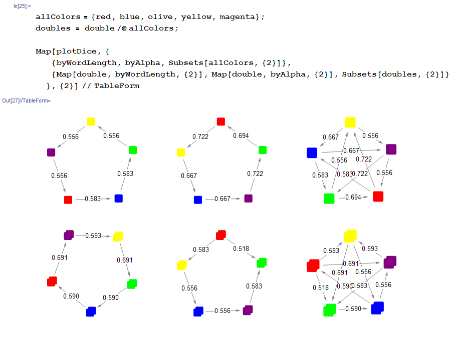
Let’s take a look at the single and double cycles visually:

Pretty neat! Besides various oddities with orientation and ordering, these plots are quite appealing. Exact placement of the vertices can be specified by the VertexCoordinateRules parameter to GraphPlot, but the default layout works well enough for our purposes.

More cycles

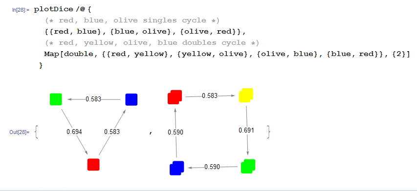
We have looked at the primary 5-color cycles using both single dice and doubles of the same color. That’s just the beginning, though.  For example, besides the 5-color cycles, various smaller cycles also exist:

How many of these smaller cycles exist? What about bigger cycles? And what about cycles involving doubles composed of 2 different colors? Or even cycles consisting of sets of 3 dice? We want to compute every possible cycle that can be created using the 10 dice from the set.

Our overall approach to solving this will be to generate directed graphs which encode all of the winning relationships between unique dice sets of a certain size (single dice, pairs, or triples), then search for cycles within those graphs.

It should be noted (we won’t prove it here) that for Grime Dice, any pair of dice beats any single die, and any triple of dice beats any pair or single die.  Thus it is indeed acceptable to split this computation up into separate buckets for single dice, pairs, and triples. There are no heterogeneous cycles with respect to number of competing dice.

Single dice

One might assume that the cycles of single dice would be the easiest to compute. In fact, single dice pose a couple of unique challenges that pairs and triples do not.  Specifically, in a set of 10 dice, we could potentially find cycles up to size 10.  But since we only have 5 colors, once a cycle becomes length-6 or longer we must necessarily have 2 same-color nodes in the cycle.  We need to make sure to differentiate between the two copies of each color.

In order to capture the fact that we have 2 copies of each color on hand, we will use a bit of a hack. The “second” copy of each color will be represented as a combination with a special “white” die which has 1 face and always rolls 0.

(* dummy "white" die used to differentiate between 
two instances of the same color die *)
white = dice["White"] = {{"White"}, {0}};

(* when plotting, just make the white die invisible *)
colors["White"] = Transparent;

(* all distinct single dice from set of 10 *)
allDice[1] = 
  Join[allColors, combine @@@ Tuples[{allColors, {white}}]];

To start building the actual relationship graph, we will define a couple of helper functions.  The first is used to create the DirectedEdge values Mathematica consumes when Graph is called in the second function.  The edges are directed from “winning di©e” to “losing di©e”.

(* Note that we don't return an edge here if the 2 dice are equally matched *)
getGraphEdge[left_, right_] := (
  {relationship, odds} = compareDice[left, right];
  If[odds != 1/2, relationship /. Rule -> DirectedEdge]
);

(* builds the graph of winning relationships for
n-tuples of dice *)
makeGraph[n_] := 
 Graph[Cases[getGraphEdge @@@ Subsets[allDice[n], {2}], DirectedEdge[__]]];

We can now generate the full graph of single dice relationships, and have Mathematica compute all cycles up to maximum size of 10.  In the last step, note that we need to deduplicate the cycle list to eliminate those cycles which are unique only due to inclusion of the dummy “white” die.

diceGraph[1] = makeGraph[1];

(* built-in function DeleteDuplicatesBy is present only
in Mathematica 10+ *)
deDupeBy[expr_, f_] := Values[GroupBy[expr, f, First]];

(* compute all cycles of single dice that can
be made from the 10 included dice *)
cycles[1] = 
  deDupeBy[FindCycle[diceGraph[1], 10, All], 
   Sort[(# /. {e_, "White"} -> {e})] &];
   
CountsBy[cycles[1], Length]
cycles[1] // Length

(* output:
  <|3 -> 5, 4 -> 5, 5 -> 2, 6 -> 15, 7 -> 20, 8 -> 20, 9 -> 10, 10 -> 3|>
  80
*)

We see that there are a total of 80 unique single-die cycles, with sizes ranging from 3 to 10.

Pairs of dice

Dice pairs turn out to be the simplest case.

With pairs (and above), we do not need to consider the possibility of distinct-yet-identical nodes in the cycle. Proof: Between any two identical nodes, there must be at least 2 other nodes (if there was only one node, it would be simultaneously beating and losing to identical nodes on either side), so a full cycle with identical nodes must have length at least 6 (the 2 identical nodes + 2 separating nodes on each side).  When each node consists of a pair of dice, this requires at least 12 dice.  Since we only have 10 dice, this is impossible.

This eliminates the need for the dummy die, as well as the de-duplication at the end.

The only additional wrinkle we need to consider is the possibility for a computed cycle to contain more than 2 dice of a particular color.  Such cycles are invalid in our scenario, since we are only utilizing the 10 dice in the set.  We will update our helpers and add some additional filtering to eliminate such cycles.

Finally, for pairs, we only need to search for cycles up to length 5.

(* all unique dice pairs *)
allDice[2] = Flatten[Table[combine @@ allColors[[{i, j}]],
    {i, 1, Length[allColors]},
    {j, i, Length[allColors]}], 1];

(* updated to avoid creating edges between nodes 
that combine to use more than 2 of any color *)
getGraphEdge[left_, right_] :=
 If[FreeQ[Tally[Join[left[[1]], right[[1]]]], {_, count_} /; count > 2],
  {relationship, odds} = compareDice[left, right];
  If[odds != 1/2, relationship /. Rule -> DirectedEdge]
 ];

(* check if a given full cycle uses more than 2 of
any particular color *)
isValidCycle[cyc_] :=
  FreeQ[Tally[Flatten[cyc /. DirectedEdge[a_, _] :> a]], {_, count_} /; count > 2];

(* compute all cycles of pairs of dice that can
be made from the 10 included dice *)
diceGraph[2] = makeGraph[2];
cycles[2] = Select[FindCycle[diceGraph[2], 5, All], isValidCycle];

CountsBy[cycles[2], Length]
cycles[2] // Length
(* output:
  <|3 -> 55, 4 -> 89, 5 -> 25|>
  169
*)

There are 169 unique cycles using pairs of dice.

Triples of Dice

Triples are the largest sets we need to consider. At least 3 nodes are required to form a cycle, and if those nodes consist of 4 or more dice each, our set of 10 dice will not be sufficient.

Similarly, we need only search for cycles of length 3 here – a cycle of 4 triples requires more dice than we have.

We start by extending our dice-combining function to handle triples, building up all such unique triples, and generating their winning relationship graph. Note that any triples where all 3 dice are the same color are invalid, and should be filtered.

(* extend to handle triples *)
combine[die1_, die2_, die3_] := combine[die1, combine[die2, die3]];

(* all unique dice triples *)
allDice[3] = Select[
   Flatten[Table[combine @@ allColors[[{i, j, k}]],
     {i, 1, Length[allColors]},
     {j, i, Length[allColors]},
     {k, j, Length[allColors]}], 2],
   Length@Union@#[[1]] != 1 &];

diceGraph[3] = makeGraph[3];

From here, computing the triple cycles should be as simple as calling FindCycle again. Unfortunately, Mathematica spins (seemingly) indefinitely when one tries this.  The relationship graph for triples is 30 nodes and 208 edges - not trivial, but not really that big. I’m not sure why FindCycle has trouble with it.  Oddly enough, FindCycle immediately finds 1 cycle if that’s all you ask for, but exhibits the hang if you ask for even just 2 cycles, let alone all of them.

So we will need to search for the 3-cycles in this graph manually. The below code does the trick.

(* for each edge in the graph, collect potential second edges
e.g. for edge A -> B, find all pairs {{A -> B, B -> X},{A -> B, B -> Y}, ...} *)
edgePairs = 
  Flatten[EdgeList[diceGraph[3]] /. 
    DirectedEdge[a_, b_] :> ({DirectedEdge[a, b], #} & /@ 
       EdgeList[diceGraph[3], DirectedEdge[b, _]]), 1];

(* find and validate the 3rd and final edge of a 3-cycle.
e.g. given {A -> B, B -> C}, check that C -> A exists, and 
the cycle A -> B -> C -> A is valid *)
completeCycle[DirectedEdge[a_, b_], DirectedEdge[c_, d_]] := (
   lastEdge = DirectedEdge[d, a];
   If[MemberQ[EdgeList[diceGraph[3]], lastEdge], (
     cycle = {DirectedEdge[a, b], DirectedEdge[c, d], lastEdge};
     If[isValidCycle[cycle],
      Sow[cycle]
     ])
   ]
);

This enables us to compute the cycles, though we do need to deduplicate them (unlike FindCycle, our manual code is not smart enough to realize the cycle A -> B -> C ->A is the same as the cycle B -> C -> A -> B).

cycles[3] = deDupeBy[Reap[Scan[completeCycle @@ # &, edgePairs]][[2, 1]], Sort];

CountsBy[cycles[3], Length]

(* output:
  <|3 -> 49|>
*)

There are 49 triple-dice cycles.  This brings the grand total to 298 unique non-transitive cycles in a set of 10 Grime Dice.

Plot all the cycles!

Finally, the fun part - making giant plots of every possible cycle!

To plot a single cycle, we just need to massage the data a little bit so that it works with plotDice from earlier.

(* 'combining' a single die is a no-op *)
combine[{name1_, vals1_}] := {name1, vals1};

(* plot a single non-transitive dice cycle *)
plotCycle[cyc_] :=
  plotDice[cyc /. DirectedEdge[l_, r_] :> {combine @@ (dice /@ l), combine @@ (dice /@ r)}];

A couple of example plots:

To generate the full plots, as linked at the top of the post, all we need is

(* plot everything! *)
plotCycle /@ cycles[1]
plotCycle /@ cycles[2]
plotCycle /@ cycles[3]